FINAL DEMOCRATIC PRIMARY PROJECTIONS: ARIZONA, IDAHO, UTAH

Sanders search interest has fallen dramatically in Arizona over the past two days, and it remains to be seen if this will have a significant impact on the results tonight, but this same rapid downward search trend happened in Minnesota and did not ultimately change anything. Meanwhile, search interest for Bernie in Idaho and Utah is through the roof. Here are my final estimates for tonight:

Screen Shot 2016-03-22 at 12.03.04 PMHillary’s greatest advantage at this time is likely all of the early ballots that have been cast in Arizona. Other states have shown us that residents who are proactive enough to cast early ballots seem to vote disproportionately for Hillary Clinton (older people, of course). Who knows if this trend will hold true in Arizona, though I imagine it will.

Here are some charts to demonstrate a few relationships between variables.

In all charts, the Y-axis is the %Vote Share of Bernie Sanders.


Screen Shot 2016-03-22 at 12.17.00 PM

The chart looking at Facebook like proportions should demonstrate that Bernie’s current “polling average” of ~23% in Arizona is not reflective of reality. Bernie almost has to land somewhere between 45% and 63% because this is such a strongly correlated variable.

Screen Shot 2016-03-22 at 12.14.28 PM

Hopefully this convinces at least a few people that what I am proposing with Arizona is not in any way a radical idea.  As you can infer from this chart, in general, Hispanics don’t tend to vote for Hillary or Bernie in America. There is actually almost perfectly no correlation.

Screen Shot 2016-03-22 at 12.11.13 PM

As for the %Black variable, and as you can see in that chart, I am actually estimating Bernie to under perform with regard to it. Bernie almost has to land somewhere between a 48% to 75% interval because this variable is also so strongly correlated with vote share.

Thanks for all of the interest,

Tyler

MICHIGAN, MISSISSIPPI DEMOCRATIC PRIMARY PROJECTIONS

It’s a bit unsettling to go against the grain with this forecast. As far as I know, every outlet is projecting a Clinton win tomorrow in both Michigan and Mississippi.

The Sanders campaign must be doing something remarkable in Michigan right now, because the upswing in Sanders popularity among my data sources is undeniable. I am seeing levels of interest in Bernie Sanders in Michigan similar to that of Colorado, Oklahoma, Kansas, and Nebraska. This, along with Michigan’s relatively normal demographic makeup, leads me to personally believe that he does have a chance. It leads my model to estimate that he will win there. Hillary leads every conventional poll, however, which makes me skeptical of these numbers.

Bernie Sanders will be lucky to get above 20% in Mississippi, but I do believe that if he doesn’t win Michigan, the final results will be very close. Here are the numbers:

Screen Shot 2016-03-07 at 11.35.52 PM

My official prediction is that Bernie will win Michigan and Hillary will win Mississippi, but in reality Michigan is too close to call with a mathematical model. Elections culminate in a single number after the movement of hundreds or thousands of variables, and as statisticians we can only select a few of those and hope that we account for as much variance as possible. Given the outcome of all the other elections so far this season, the positions of those variables right now in Michigan seem to indicate that a massive upset will happen tomorrow night.

-Tyler

KANSAS, LOUISIANA, NEBRASKA, MAINE DEMOCRATIC PRIMARY/CAUCUS PROJECTIONS

After projecting one incorrect result on Super Tuesday, in the state of Minnesota, I was able to refine my forecasting models further. There does seem to be some variability in these outcomes that I am currently unable to account for, e.g. if the models predict a win in Minnesota, a win in Iowa also should have happened. Iowa could without a doubt be a special case for our purposes, as it was indeed the first state to hold a Democratic Caucus, both candidates had been campaigning there relentlessly for months, and so on. Therefore, it stands to reason that, looking backwards, perhaps it was Iowa that was the anomaly, and not Minnesota. Sanders outperformed my estimates in every state except Texas, Alabama, and Arkansas; with these states of course having in common the characteristic of being southern and having a larger minority population.

Fortunately, these next four states seem to be firmly in one or the other candidate’s favor. Here are the new projections:

Screen Shot 2016-03-04 at 9.35.51 PM

Hillary Clinton will win Louisiana by a significant margin, but the subtle and interesting characteristic of this estimate (as my colleague Matt pointed out to me) is that the estimated margin of victory seems to be smaller than other similar states. For instance, Georgia, Alabama, and South Carolina are almost identical in demographic makeup as Louisiana, yet Clinton won all those states with greater than 70% of the vote. This could signal that Bernie Sanders is becoming increasingly more popular with the minority community.

Bernie Sanders is projected to win the other three states, Kansas, Nebraska, and Maine. Though these states have relatively few delegates up for grabs, this will still be a victory for his campaign insofar that it should create some positive momentum for his campaign after he lost the majority of the Super Tuesday states. Honestly, I expected the estimates for Kansas and Nebraska to signal a more hotly contested race, but the data from the past three days shows that the residents of these states are certainly feeling the Bern.

Special thanks to Andrew, Phil, and Matt for their collaboration and thoughts.

-Tyler

SUPER TUESDAY DEMOCRATIC PRIMARY AND CAUCUS PROJECTIONS: REVISED

It has become clear that the social media data that I used in my previous forecast became antiquated quite quickly, due to the relatively large margin between the South Carolina estimate and actual result.

Thanks to a good friend’s tip, I began to utilize data from Google Trends to develop new estimates for Super Tuesday. Looking in retrospect, the correlation between the Google data and results in the first four states is striking once one has massaged the data set to produce usable measures (I use relative search frequency averaged over the couple days prior to the election). Demographics are taken into account as well. The new estimates are as follows:

Screen Shot 2016-03-01 at 12.22.32 AM

This produces an estimated delegate allocation as follows (super-delegates are not included in this table):

Screen Shot 2016-03-01 at 12.27.15 AM

Once we have the data from Super Tuesday, we will all be able to hone the accuracy of our models even further.

-Tyler

IOWA SENATE RACE 2014

The 2014 Iowa Senate race was a hard-fought campaign between two individuals that had vastly different visions for the future of America. In the red corner was Joni Ernst, a former lieutenant colonel in the National Guard and a member of the Iowa Senate. Ernst’s political career had been running smoothly and had been developing momentum since she was elected Montgomery County Auditor in 2004. In the blue corner was Bruce Braley, a member of the U.S. House of Representatives and successful trial lawyer. Braley had served in Congress since 2007, and it was time for him to take the next step: the U.S. Senate.

Unfortunately for Braley this dream didn’t work out in his favor, but why? How can a U.S. Representative that has been consistently reelected by large margins lose to a relatively new member of the Iowa Senate that wasn’t initially electorally popular for any reason other than one television advertisement? The importance of this election is not to be understated, as it was viewed nationally as the central indicator as to whether the Republican Party would take control of the U.S. Senate.
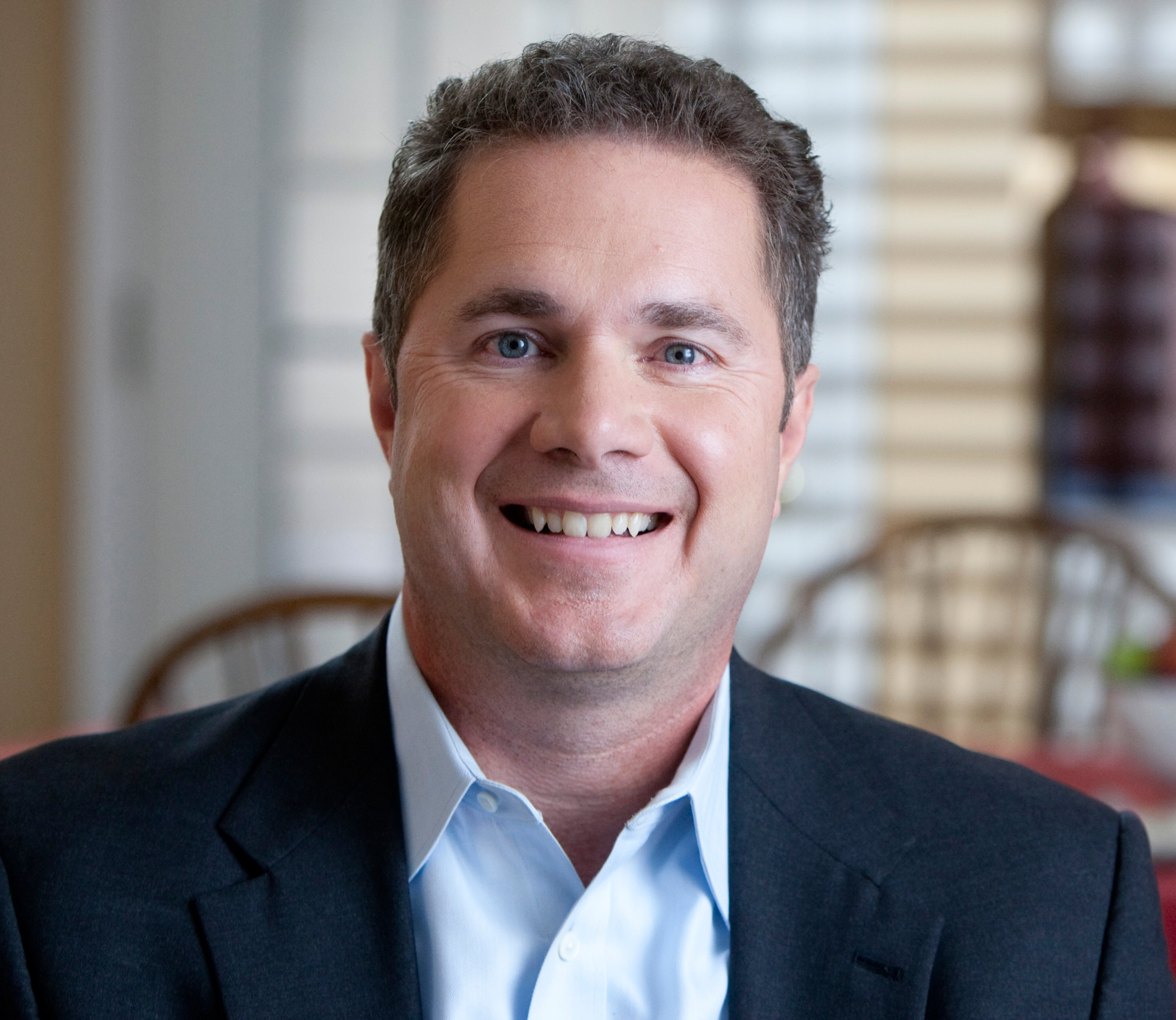
BRUCE BRALEY

Iowa has historically been a conservative state, often electing Republicans to Congress. In fact, in the entire history of Iowa, Iowans have sent 27 Republicans to the Senate, and only 11 Democrats. The Iowan delegation to the House of Representatives is not much different, 154 Republicans to 54 Democrats, with the Democrats usually serving far shorter terms. However, the recent trend indicates a far more purple political reality in Iowa. Democrats have made a fair amount of progress within the past few decades, with some districts turning blue and sending Democrats to Washington much more often than history would have us predict. This leads us to speculate whether the red wave of November 2014 was a bonafide partisan shift, or merely a product of temporary circumstance; attributable to the presidential party backlash almost always seen during a mid-term election cycle.

Braley-HR-Headshot

Bruce Braley was part of this recent Democrat progress, coming in with the wave of Democrats that were elected as the American financial sector was crumbling in 2006, beating out Republican Mike Whalen by a comfortable 12% margin (BallotPedia, 2014). Democrats have struggled to maintain this advantage after taking control of all three branches of government at the federal level, but due to the unpopularity of the Affordable Care Act, Republicans have now erased all of the aforementioned Democrat gains and more. Bruce Braley was one of the few new Democrats remaining in 2014; with “new Democrats” being defined as Democrats that came from otherwise conservative congressional districts that were only elected out of voter disdain for the Afghanistan and Iraq wars in the mid 2000’s. After all, Braley’s 1st Congressional District seat in the U.S. House had been controlled by Republicans for 89 of the previous 101 years prior to his first victory (Office of the Clerk, 2015). Perhaps it was that Braley underestimated current voter disdain President Obama and anyone that was a member of the Democratic Party. Braley was hanging onto his House seat in a historically very conservative district, but he assuredly did not have the prospect of Tom Harkin’s Senate seat locked down. However, the stars aligned and gave Braley arguably the best chance he would get to take this step up, presenting him with a mediocre Republican field and plenty of leftover 2012 campaign funds to take his shot.

Braley attended Iowa State University in his youth, and received his Juris Doctor from the University of Iowa College of Law. After this, he started his long career as a trial lawyer, and following his Senate campaign loss, now litigates full time once again. In the years leading up to 2014, he had taken steps to eventually prepare himself for the Senate. In 2006 Braley won his first campaign by a significant margin, 55.1% to 43.2%, after the 1st congressional district seat was vacated. He followed this up with another win, 64.6% to 35.4% in 2008, 49.5% to 47.5% in 2010, and 56.9% to 41.6% in 2012. His constituents had, for the most part, decisively (with the exception of 2010) chosen him to represent them. Fortunately for him, in his run for Senate in 2014, Braley faced no opposition in the primary (BallotPedia, 2014).

Polling long before the primaries, in 2013 and early 2014 steadily showed Braley with a decisive lead to the tune of 6%-12%. He had established name recognition, a proven campaign organization, and no challenge in the primary, which gave him an advantage over whoever his opposition would eventually be. Because of this, Braley only had to run a textbook campaign. There was no need to be inventive, to experiment with anything new, or for him to even begin running negative campaign advertisements about Ernst. With his early lead and plenty of campaign funds, he was comfortable going into the race. It wasn’t until Ernst had won the Republican primary, and her organization released a video of Braley making a questionable comment about farmers, that he began to lose ground. In early June, polls began to show Braley trailing Ernst as negative campaign ads flooded Iowans’ TVs. Braley’s advantageous position had been completely eliminated, and the status quo had been turned upon its head. A textbook campaign would no longer suffice, and he would find it necessary to resort to more incendiary campaign strategies, like negative ads about Ernst, to defend himself. Voters now had video evidence that Braley may not be who he claims to be, and the Braley campaign found it easier to defame Ernst rather than attempt to erase negative perceptions of Braley from the voters’ minds. This new foundation created a far more volatile campaign, and from June until Election Day, the race was a complete toss-up with practically each subsequent poll showing a different candidate in the lead (Real Clear Politics, 2014).

  Screen Shot 2015-05-03 at 3.39.03 PMSource: Real Clear Politics, 2014

The aforementioned “comment” was a remark he made about Iowa Senator Chuck Grassley, and this early misstep eroded much of the fundamental advantage he had going into the election. Braley hosted a fundraiser for his Senate campaign in January 2014, and invited fellow attorneys in an attempt to persuade them to donate to his cause. He cited his prospective appointment to the Senate Judiciary Committee, and his background in law; implying that he would ensure that the Senate didn’t pass any legislation that would be harmful to lawyers’ practice, saying, “If you help me win this race, you may have someone with your background, your experience, your voice … on the Senate Judiciary Committee. Or you might have a farmer from Iowa who never went to law school, never practiced law, serving as the next chair of the Senate Judiciary Committee.” A video of Braley making these comments was released by a conservative political action committee, America Rising, and his opposition ruthlessly capitalized on his poor choice of words for the entirety of the campaign. Despite apologizing to Senator Grassley and the public, Braley never recovered from this mishap (Lachman, 2014). Iowa has a massive amount of agricultural, and naturally a large population of farmers. Braley’s comment taken out of context looks like an obvious attack on farmers’ intelligence, when in fact it is clear that he meant that farmers don’t typically have an education in public law and the judicial process, and that an attorney would be better suited to serve on the Senate Judiciary Committee, which is a fair assertion to make. However, no amount of apologies would have erased the damage he had done to his campaign.

Braley’s obvious strength is the connections he has and his ability to fundraise. Money was of no shortage to him, and “At the end of 2013, Braley had more than $2.6 million in his campaign account,” (Sullivan, 2014). In total, Braley raised $12,082,748 for the campaign, with 77% coming from itemized and un-itemized individual contributions (Federal Election Commission, 2014). His early money put him in a great position to control how he wanted his campaign message to emerge, and to what magnitude he wanted his campaign to have a presence in Iowa early on. However, because of his Grassley comment, he was thrust into the spotlight much earlier than he had anticipated, and was forced to start burning money to erase the negative image voters had about him. In retrospect, it may be safe to say that he should’ve let the gaffe fizzle out and not spend money trying to refute what the opposition was saying, but this knee-jerk spending reaction can nonetheless be perceived as a reasonable course of action to have taken given the circumstances.

Screen Shot 2015-04-14 at 9.48.49 PMSource: Center for Responsive Politics, 2014

            As for outside spending, there was a total of $23,751,533 in money coming from outside the state that was spend on Bruce Braley, with $4,244,593 spent in support of him, and $18,841,528 opposed to him (Center for Responsive Politics, 2014).

JONI ERNST

Joni Ernst, Montgomery County native, attended Iowa State University and joined the National Guard after her graduation. She was deployed during the Iraq war in 2003 and led 150 other servicemen and women in Kuwait and Iraq as a Lieutenant Colonel (Ernst, 2015). These credentials helped to give her campaign something tangible for voters to rally around, and certainly bolstered her position relative to her opponent Bruce Braley. She won her seat in the Iowa State Senate in 2011 in a special election after the seat was vacated with an impressive 67.4% of the vote, spending $128,208 to win it. She was subsequently reelected in 2012 when she ran unopposed. Ernst has since served on various committees, which helped to build momentum behind her as a rising star in the Republican Party (Ballotpedia, 2014).

140929_POL_JoniErnst.jpg.CROP.promo-mediumlargeErnst faced a difficult Republican primary in the 2014 Senate race. There were five total contenders, and being a new face in the Iowa legislature, she didn’t necessarily have much to differentiate herself from the rest of the pack. Her competition was famous, qualified, and well funded. Among them were the former CEO of an energy company Mark Jacobs, the popular radio host Sam Clovis, the former U.S. Attorney Matt Whitaker, and Scott Schaben.

Ernst had largely trailed the pack until she released her famous “Squeal” advertisement in March of 2014 which was an instant success and received national attention due to the content of the commercial, in which she says “I can castrate pigs so I am the perfect conservative for Iowa to send to the Senate . . . I grew up castrating hogs on an Iowa farm. So when I get to Washington, I’ll know how to cut pork. Washington’s full of big spenders. Let’s make ’em squeal.” The voters loved the message, as Ernst perpetuated the state-versus-federal narrative that so many citizens enjoy hearing. This and one other clever commercial gave Ernst instant notoriety, and she led the polls until Election Day, ultimately winning with 56.2% of the vote (Ballotpedia, 2014).

Screen Shot 2015-05-03 at 3.01.22 PMSource: Real Clear Politics, 2014

Jacobs, overall, raised a staggering $3.1 million for the primary campaign; eclipsing the $1 million Ernst raised which is neither a small sum (Hohmann, 2014). Unfortunately for Mark Jacobs, his $3.1 million only bought him 16.8% of the vote. Clovis, despite raising only $282,000, ultimately came in second place with 18% of the vote share; no where close to Ernst’s impressive 56.2% (Hayworth, 2014). Matt Whitaker captured 7.5%, and Scott Schaben came out with 1.4% of the vote.

Immediately following her victory in the primary, Ernst’s backers began ruthlessly advertising Braley’s January gaffe. Negative campaigning was a central strategy employed by both camps during this race, but Ernst’s campaign used it far more; but this was largely because Braley gave them more material to use. Indeed, Ernst ran an airtight campaign, with no slip-ups that ever became heavily publicized. Braley had to resort to criticizing her for who was donating to her and her stances on issues. However, Braley was not wrong to lambast her on her political positions, as this was the only real Achilles heel of Ernst’s campaign; she holds very atypical views, far more inline with the Tea Party than the mainstream Republicans, even on issues where the people are in nearly universal agreement. Ernst supports repealing the federal minimum wage, disbanding the Department of Education, disbanding the Environmental Protection Agency, repealing the Clean Water Act, banning abortion, and much more (KCCI, 2014). For Braley and nearly any other candidate that has run a campaign, Ernst’s positions could be considered ripe to be taken advantage of and exploited to discredit her to the electorate.

The Affordable Care Act (ACA), one of the most salient political issues at the time, was addressed on several occasions, but mostly in TV advertisements. Braley supported the legislation as whole, but thought there was room for improvement. Ernst repeatedly called for the repeal of the Act and the dismantling of the state and federal exchanges (KCCI, 2014). Whether each candidate truly believed in the stances they took, we will never know, but each position did play to each base appropriately. Because the ACA was so divisive at the time of the election, the Braley campaign steered clear from initiating the debate on it. Every occasion that it was introduced as the topic of discussion was initiated by Ernst campaign, and rightfully so.

Despite their very clear positions on the main issues in contemporary American politics, issues are not what decided this election. Joni Ernst has an impressive natural charisma. She has a Clinton-like personality, insofar that she is likable, charming, and very pleasant to listen to if you are any average voter that is looking for reasons to like a candidate. Ernst possesses a personality characteristic that allows her to make a connection with voters on a personal level; something the Bruce Braley tended to lack when he needed it most. When you set aside the politics, she was just simply more likable, and had a personal touch that couldn’t be matched by Braley.

Additionally, Ernst showed promise in the fundraising realm, despite many having doubts that traditional conservatives throughout the country would throw their money behind a newcomer, and furthermore a newcomer that had such Tea Party reminiscent positions on the issues. Ernst raised a total of $12,011,101, with 80.1% coming from individual contributions, a very impressive feat. But, because she had a primary to deal with, by the time she reached the general election campaign she had already spent $461,206.00 (Federal Election Commission, 2014). This and Braley already having $2,600,000 in his war chest put Ernst at a disadvantage, and forced her to raise more money, and to make what money she had go further. There was a total of $37,544,557 in money coming from outside the state that was spent on Joni Ernst, with $12,244,939 in support of her, and $25,196,618 opposed to her (Center for Responsive Politics, 2014).

Screen Shot 2015-04-14 at 9.50.10 PMSource: Center for Responsive Politics, 2014

OUTCOME

A recurring theme in the Iowa Senate race was both sides accusing each other of receiving money from billionaires. For Braley, there were many advertisements that aired informing voters of Ernst’s ties with the billionaire Koch brothers. He called Ernst out on that personally during their debate when asked about renewable fuel standards, saying, “I’m not sure that’s what Senator Ernst told the Koch brothers when she went to their secret meetings.” From Ernst, there were countless advertisements telling voters that Braley had taken money from billionaire Tom Steyer, and she also personally called him out on it during their debate in response to Braley’s claim, saying, “You are being funded by Tom Steyer, who is a Californian billionaire extreme environmentalist,” (KCCI, 2014). All in all, this strategy for both sides was a zero-sum game, and it was not a wise strategy for Braley to employ. He should have known that Ernst could refute his point in the way that she did. Once Braley had made the original claim, Ernst’s hands were tied, and she was forced to call Braley out on his connection with Tom Steyer. Braley was the pot that called the kettle black.

Regardless of how effective of a legislator Bruce Braley was, the reality of his tenure as a U.S. Representative is that he was originally elected during the Democrat wave of 2006, in which the party picked up thirty-one seats in the House (The New York Times, 2006). Thus, if an unpopular President Bush got him elected, an unpopular President Obama certainly wasn’t helping his cause this go-around. Republicans have applied relentless pressure since the massive gains the Democrats made in 2006 and 2008, rooting out all of the new democrats that found a seat during the Great Recession. From this perspective, Bruce Braley actually held onto his seat far longer than many of his fellows that got the boot when the public revolted in 2010 and gave the Republicans sixty-three new House seats. If nothing else, the fact that Bruce Braley is the longest serving Democrat in the history of the Iowan 1st Congressional District (dating back to 1845) is proof enough that he has either represented his district extremely well, or that he exploited a temporary wave of liberal sentiment very well. Whatever the reason, the people in his district were happy with him being their representation in Washington D.C. for the better half of a decade.

Iowa is demographically one of the least diverse states in the nation. Whites comprise 88.3% of the population compared to 64.2% nationally, while Blacks account for just 3.0% compared with 12.2% nationally (County Health Rankings, 2015). Of the 3,074,186 people that live in Iowa, 2,142,304 are registered to vote as of November 2014, giving Iowa a 69.6% registration rate (Iowa Secretary of State, 2014). This actually puts Iowa in the better half of the country for voter registration rate, 13th, as of 2012 (Pew Charitable Trusts, 2014). As for turnout in 2014, the turnout in Iowa was 50.2%, 7th highest in the nation. This is likely attributable to not only the highly contested race, but also because Iowa allows for same-day voter registration (Nonprofit VOTE, 2015). There is no doubt that Iowa’s relatively high mid-term turnout helped Bruce Braley, and there is also no doubt that Iowa’s extremely low black population helped Joni Ernst. The lack of a diverse population is relatively unique to Iowa and few other states, and this is one metric that makes it more difficult for Democratic candidates to win in the state. Though to be fair, this demographic composition has obviously not been the source of any electoral trouble for Braley in years past.

Joni Ernst was also successful in turning the Iowa Senate race into an “Iowa versus Washington” race, and was arguably her central goal and campaign strategy. Ernst consistently returned to this theme, forcing Braley to spend his valuable time trying to refute the notion that he was a part of the inoperative Washington machine to the point of almost trying to convince voters that he wasn’t a member of Congress. Embodying this central strategy of Ernst’s is a statement she gave immediately after she won the primary, saying “This campaign will come down to a very simple choice: our shared Iowa values, versus Bruce Braley’s liberal Washington values,” (Politico, 2014).

CONCLUSION

The 2014 Iowa Senate race can be summarized as follows: Bruce Braley may have been the more experienced legislator, but Joni Ernst knew how to campaign better. This touches on an interesting phenomenon in political science; that it takes a different set of skills to get elected to legislate than it does to legislate, and because of this, sometimes individuals who aren’t suited for the actual work are the ones that win elections. Joni Ernst was better able to connect with the voters by simplifying the issues down to digestible chunks of information. She’s charismatic and influential. Bruce Braley seems to have an outstanding grasp on the specifics of the issues and a more mainstream average position on the current issues that matter and issues Ernst created, but seemed standoffish and un-relatable enough to make voters remember him for it.

Braley may not have been able to survive the “red tide” no matter what happened, but the quality of his campaign in contrast to Ernst’s certainly made it impossible. Ernst turned Braley into an outsider, and convinced voters that he was completely disconnected with the reality of their shared condition.

-Tyler

REFERENCES

BallotPedia. (2014). Bruce Braley. Retrieved April 11, 2015, from BallotPedia: http://ballotpedia.org/Bruce_Braley

Ballotpedia. (2014, November). Joni Ernst. Retrieved April 14, 2015, from Ballotpedia: http://ballotpedia.org/Joni_Ernst

Center for Responsive Politics. (2014, November). Rep. Bruce Braley. Retrieved April 12, 2015, from OpenSecrets.org: https://www.opensecrets.org/politicians/industries.php?cycle=2014&cid=N00027464

County Health Rankings. (2015). 2015 Iowa Summary Report. University of Wisconsin. Madison: County Health Rankings.

Ernst, J. (2015, January). About Joni. Retrieved April 14, 2015, from Joni Ernst – United States Senator: http://www.ernst.senate.gov/content/about-joni

Federal Election Commission. (2014, November). Details for Candidate ID: S4IA00087. Retrieved April 12, 2015, from Federal Election Commission: http://fec.gov/fecviewer/CandidateCommitteeDetail.do

Hayworth, B. (2014, June 4). Clovis Looks Back on Iowa Primary Loss. Retrieved May 2, 2015, from Sioux City Journal: http://siouxcityjournal.com/news/local/a1/clovis-looks-back-on-iowa-primary-loss/

Hohmann. (2014, June 3). Joni Ernst wins Iowa GOP Senate Primary. Retrieved May 3, 2015, from Politico: http://www.politico.com/story/2014/06/joni-ernst-iowa-gop-senate-primary-2014-elections-bruce-braley-107401.html

Iowa Secretary of State. (2014). State of Iowa Voter Registration Totals. Des Moines: State of Iowa.

KCCI. (2014, September 28). Iowa U.S. Senate Debate. Retrieved April 7, 2015, from Youtube: https://www.youtube.com/watch?v=NOUodSNyZtg

Lachman, S. (2014, March 26). Bruce Braley Faces Harsh Criticism In Iowa Over Farmer Comments. Retrieved April 11, 2015, from Huffington Post: http://www.huffingtonpost.com/2014/03/26/bruce-braley-iowa_n_5034847.html

Nonprofit VOTE. (2015). America Goes to the Polls 2014. Nonprofit VOTE.

Office of the Clerk. (2015). Election Statistics. Retrieved May 3, 2015, from Office of the Clerk – U.S. House of Representatives: http://clerk.house.gov/member_info/electioninfo/index.aspx

Pew Charitable Trusts. (2014, April 8). Elections Performance Index. Retrieved April 12, 2015, from Pew Trusts: http://www.pewtrusts.org/en/multimedia/data-visualizations/2014/elections-performance-index#state-IA

Politico. (2014, June 3). Joni Ernst wins Iowa GOP Senate Primary. Retrieved April 10, 2015, from Politico: http://www.politico.com/story/2014/06/joni-ernst-iowa-gop-senate-primary-2014-elections-bruce-braley-107401.html

Real Clear Politics. (2014, Novmeber 4). Iowa Senate – Ernst vs. Braley. Retrieved April 11, 2015, from Real Clear Politics: http://www.realclearpolitics.com/epolls/2014/senate/ia/iowa_senate_ernst_vs_braley-3990.html

Sullivan, S. (2014, April 3). Bruce Braley’s bad week. Retrieved April 11, 2015, from The Washington Post: http://www.washingtonpost.com/blogs/the-fix/wp/2014/04/03/how-angry-farmers-could-help-the-gop-win-back-the-senate/

The New York Times. (2006, November 4). 2006 Election Guide. Retrieved April 10, 2015, from The New York Times: http://www.nytimes.com/ref/washington/2006ELECTIONGUIDE.html
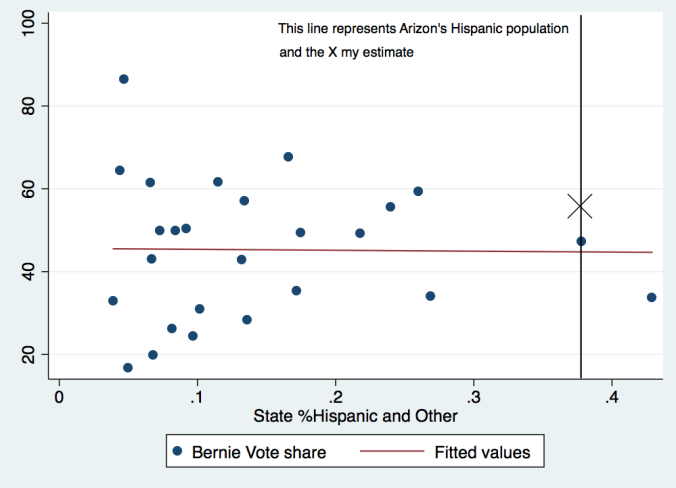
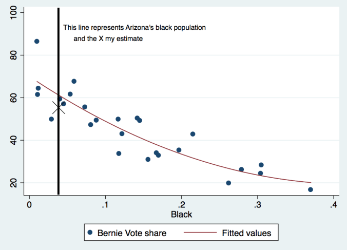
DO VOTERS HOLD THE PRESIDENT AND GOVERNORS ACCOUNTABLE TO ECONOMIC PERFORMANCE? NOT REALLY.

INTRODUCTION

There are a multitude of factors that dictate how someone votes in an election, and for a large share of individuals, whether they even vote at all. Political Science has a long history of attempting to define which characteristics influence the electorate to vote for a particular party; sometimes for academic purposes, but in the election industry, these defining characteristics are very valuable information.

There are internal factors and external factors that decide an individual’s vote. Internal factors are characteristics inherent to the person that increases their predisposition to vote for a particular political party, e.g. race, sex, or age. External factors are things that occur out in society that influence an individual’s political leanings, e.g. the salience of a social issue at the time of the election, economic growth or shrinkage, or the response of an administration to a national security threat. The effects of these events on the electorate are more difficult to quantify, but that is the aim of this paper, at least for one specific type of external factor: economic growth.

Do voters hold government officials, more specifically executives, accountable to economic performance during their tenure? What about the party of the executive; do voters punish the political party of the executive when economic performance is poor and reward it when it exceeds expectations? At first the answer seems like an obvious one. In fact, if there were any factor that did dictate the electorate’s vote, it would seem that most would say economic performance was it. But, the interesting part of this lies in the specifics, and implications of the question. If it is found that economic performance has little to no bearing on the electorate’s aggregate vote for the political party that is in power at the executive level, then this would indicate that voters do not make their decision in the context of political parties. Perhaps it would mean that they place more emphasis on the personal characteristics of the candidate. Alternatively, it could indicate that the partisan divide is so strong that voters, on the aggregate level, vote on party lines despite how good or bad the perceived economic leadership of the president or governor is during their tenure. And lastly, it could even indicate that campaigns are so effective at pushing a specific narrative that voters forget the reality of economic conditions.

But what results do you get when you examine the relationship between state economic conditions and presidential vote share? Do voters hold the president’s party accountable, and furthermore do they hold the president’s party accountable for state economic conditions that are outside of the national government’s control? In this paper we will discover whether or not a relationship exists, and determine whether or not accountability stays in its appropriate sphere. Building on this as well, we can make some determinations of other factors that affect presidential and gubernatorial success in elections.

RELEVANT RESEARCH

            Nearly every publication in political science regarding this subject looks at election results through the lens of two different voting behavior models. The first is the national referendum model, which “suggests that voters in subpresidential elections express their approval or disapproval of the sitting president and his policies with their vote.” The other model is the economic voting hypothesis, which “suggests that voters in these elections express support or dissent for the performance of the incumbent based upon how well the economy is doing,” (Atkeson and Partin, 1995). At its core, this last model indicates that voters who are financially better off than they were before the candidate took office will reward the incumbent, and conversely will punish them if that does not hold true. The economic voting hypothesis is what we are primarily taking a look at here, with a couple of variables that would shed some meaningful light on the applicability of the national referendum model in the gubernatorial analysis.

Institutions, The Economy, and the Dynamics of State Elections takes a deep look into the aforementioned topic at the state legislative and gubernatorial levels (Chubb, 1984). Chubb considers the relative effects of presidential coattails, the common backlash against the party of the president during mid-term elections, and state and national economic conditions. He believes that “. . . when it comes to assigning responsibility for economic performance, state voters have generally and increasingly looked outside of the state to the national economy and the president’s imputed performance in managing it,” thus a poorly performing national economy would influence the outcome of a state election, despite a state’s hypothetical independently strong economic performance. The analysis of this paper has shown Chubb’s claim to be inconsistent with voting behavior in the last two decades, but perhaps there has been a genuine change in behavior between the time period he analyzed and now. Lastly, Chubb says that at the state level, “the factors that account for variations in normal partisan voting across the states include idiosyncrasies of culture and history that subvert general explanations,” which corroborates the findings of the analysis here. Gubernatorial electoral outcomes are the product of far more variables than presidential electoral outcomes.

James King, of the University of Wyoming, in 2001 performed a similar analysis in his publication titled Incumbent Popularity and Vote Choice in Gubernatorial Elections. Studying gubernatorial elections in four states, his results found that “. . . voters use the ballot for governor to express approval or disapproval of current economic conditions and the president’s job performance, or as an easy means of evaluating candidates.” This would square with Chubb’s publication that retrospective economic voting is a reality, and that voters hold the governor accountable to state economic performance.

Atkeson and Partin, in Economic and Referendum Voting: A Comparison of Gubernatorial and Senatorial Elections come to similar conclusions. They find that “. . . governors, as chief executives of their respective states, are held responsible for the health of their state economies and are not generally shown to be liable for fluctuations in presidential approval.” This further affirms the existence of economic retrospective voting at the gubernatorial level. Atkeson and Partin also “. . . find something of an in-party incumbency effect whereby incumbent governors of the president’s party suffer more from a perceived worsening of state economic conditions than incumbents of the out party,” and finally they claim, “. . . governors . . . escape from these national-level evaluations of presidential performance and are instead held liable for state economic conditions.” This would suggest that national economic performance has no bearing on governors, regardless of political affiliation.

In a very interesting article written by Robert M. Stein in 1990, the argument is made that economic conditions affect presidential vote share, but not gubernatorial, saying “. . . state and local incumbents are less likely to be affected by voters’ retrospective economic evaluations than their national counterparts.” Stein’s usage of the word “incumbents” would indicate that voters do not punish or reward the incumbent party when an incumbent is term limited and the election is open-seat. Stein’s findings do confirm his aforementioned hypothesis, and he goes on to state that “Voters hold their governor neither responsible nor accountable for the state’s economic conditions and their voting behavior reflects this perception . . . This evidence of economic voting for governor, however, varies with the partisan affiliation of the incumbent candidate,” thus when economic effects do matter in an election, voters will punish or reward each party by different amounts for the same economic performance. Stein’s research shows that voters differentiate between the impact state and federal policies can have on their personal finances, wrapping up his article by saying that “voters recognize that their personal financial condition is more closely tied to federal policies and actions than to the state’s,” (Stein, 1990).

A different approach to testing the executive economic accountability theory is taken by David Samuels and Timothy Hellwig. They cited the controversy of trying to define the dependent variable in the accountability model; whether to measure accountability as number of seats in a legislature swings in vote share of an incumbent, or in its most stringent sense, partisan control of the office in question. They found that accountability can be observed when measuring it as seats in a legislature or vote share of an incumbent, saying “When we conceive accountability in terms of sensitivity of swings in incumbent vote shares . . . and when we use seats as the dependent variable, we find that incumbent performance is sensitive to economic performance.” However, when measuring accountability as partisan control of the office, the results were inconclusive, saying “. . . when we conceive of accountability as partisan control over government . . . our findings temper Cheibub and Przeworski’s (1999) pessimism.” The authors ultimate conclude that “citizen control of politicians is . . . imperfect because particular political contexts limit voters’ ability to hold incumbents to account by obscuring responsibility for economic performance,” (Samuels & Timothy, 2010).

Johnson and Ryu look to other countries to test these models, but with the inclusion of broken campaign promises in the analysis. They sought to determine if economic performance, broken promises, or some combination of the two were what voters cared most about in executive elections. Their findings indicated that neither of the two factors had any substantive effect alone, but an interaction between both variables resulted in statistically significant results, going on to say that “the relationship between broken campaign promises and incumbent vote change is affected by economic conditions.” This means that regardless of economic performance, as long as no campaign promise was broken, the executive was not rewarded nor were they punished for it; and alternatively, when a campaign promise was broken, voters held the executive accountable for economic performance, likely due to increased scrutiny (Johnson & Ryu, 2007).

METHODOLOGY

Data was gathered from official and private sources (deferring to official whenever possible), from the years 1987 to 2013.

The hypothesis for the state level is as follows:

 State Level H1: People vote to retain the governor, or party of the governor when he/she is term limited, when the state in question experiences strong economic growth.

State Level H2: On average, a governor will be positively affected when the governor is the same political party as the sitting president and their elections coincide.

The overall theorized model of the analysis is specified by the following regression equation:

 %VoteShareGovParty = β0 + β1 % StateGrowth + β2 % NationalGrowthSamePres – β3 %NationalGrowthOppPres + β4 PartisanControl + β5 GovIsIncumbent + β6 GovSamePartyElectionasPres + ε

The following are variable definitions:

%VoteShareGovParty: The percentage of vote share received by the party of the incumbent governor, whether the governor was running for reelection or not.

%StateGrowth: Measured as the percentage change in Per Capita Real Gross State Product over the tenure of the governor.

%NationalGrowthSamePres: An interaction between a dummy variable that turns on when a governor is the same party as the president, and the percentage change in Real Gross Domestic Product

%NationalGrowthOppPres: An interaction between a dummy variable that turns on when a governor is the opposite party as the president, and the percentage change in Real Gross Domestic Product

PartisanControl: Serves as a baseline for the predicted vote share of a governor. This is measured by taking the average of the vote share of the Democrat Party for every gubernatorial election between 1987 and 2013, and providing that number if the incumbent party is Democrat, or 100 minus that number if the Incumbent party is Republican. The coefficient of this variable will be difficult to interpret, and is not meaningful for our sake.

GovIsIncumbent: This is a dummy variable that turns on if the governor is an incumbent.

GovSamePartyElectionasPres: This is a dummy variable that turns on if the governor is the same party as the president, and their elections fall on the same year.

Gubernatorial election results and information on gubernatorial incumbency were aggregated from Wikipedia, which has curated lists that source the data from each state’s secretary of state or equivalent. I am aware that Wikipedia is frowned on to use as a source in an academic context, but there was simply no other source that had the data in a remotely useful format. National RDGP growth, as well as state per capita RGDP growth figures were obtained from the Bureau of Economic Analysis. The rest of the variables were computed through Excel functions to prepare the dataset. Observations were discarded if the incumbent party was not Democrat or Republican, and after the completion of the dataset, there were 327 total observations being analyzed. For the regression analysis, Stata 14 was used.

The national level model is much the same, with two hypotheses as well:

National H3: People vote to retain the president, or party of the president when he is term limited, when the country as a whole experiences strong economic growth.

National H4: People vote to retain the president, or party of the president when he is term limited, when their state experiences strong economic growth.

The overall theorized model of the analysis is specified by the following regression equation:

%VoteSharePresParty = β0 + β1 % StateGrowth + β2 % NationalGrowth + β3 PartisanControl + β4 PresIsIncumbent + ε

The following are variable definitions:

%VoteSharePresParty: The percentage of vote share received by the party of the incumbent president, whether the president was running for reelection or not.

%StateGrowth: Measured as the percentage change in Per Capita Real Gross State Product over the previous presidential term.

%NationalGrowth: Measured as the percentage change in Real Gross Domestic Product

PartisanControl: Serves as a baseline for the predicted vote share of a president. This is measured by taking the average of the vote share of the Democrat Party for every presidential election between 1987 and 2013 and for every state, and providing that number if the incumbent party is Democrat, or 100 minus that number if the Incumbent party is Republican. Like the gubernatorial model, the coefficient of this variable will be difficult to interpret, and is not meaningful for our sake.

PresIsIncumbent: This is a dummy variable that turns on if the president is an incumbent.

Presidential election results and incumbency information were aggregated from The American Presidency Project. National RDGP growth, as well as state per capita RGDP growth figures were obtained from the Bureau of Economic Analysis. The partisan control variable was computed through excel functions. Observations were adjusted if there was a third party candidate to exclude that impact on the results.

DISCUSSION

Screen Shot 2015-05-07 at 8.27.16 PM

After running the regression analysis on the data and ensuring that there were no omitted variables, we are presented with some very interesting results. Three different models were created for the gubernatorial level, with each subsequent model adding controls in an attempt to isolate the real effects that state GDP growth and national GDP growth have on the vote share for the political party that is in power at the executive level in state government. Though no heteroscedastic problems were foreseen, every model was controlled for heteroscedasticity by using the robust command in Stata. Refer to Table 1 for the results of all three models.

Screen Shot 2015-05-07 at 8.27.06 PM

After producing a correlation matrix, we find no possible issues with multicollinearity in the model. Notice the low correlation between the PartisanControl variable and %VoteShareGovParty. The PartisanControl variable takes historical voting averages for the Democrat Party in each state and uses that number as a baseline to predict vote share in the year in question. However, because aggregate state partisanship is much more volatile than the country as whole, and is susceptible to much quicker political ideology shift, historical voting averages are not nearly as good of a baseline at the state level as they are for the national level. In an ideal world, this correlation number would be equal to 1.000, which would allow us to perfectly predict the outcome of each election with only one piece of data, but unfortunately this is not the case. As you will soon see, the presidential model correlation between these two variables was much higher, leading to a much more accurate model.

Neither state nor national economic performance has any effect on gubernatorial vote, and we cannot accept H1. The closest either variable gets to any significance is with a p-value of 0.102, but even this is in Model 1 when the other controls are not active. This is a surprising result, and though the p-values for the state, same-party-national and different-party-national variables are 0.335, 0.995 and 0.736 respectively in the complete model, the R2 is 0.429. This means that there are other variables out there that will account for the other 57.1% of the variance in vote share for the political party in power. If those were controlled for, there is a chance that state and national economic performance could come back down into significance. However, the challenge with this is that there is no shortage of unobservable variables that have some bearing on the outcomes of elections.

To those familiar with the field of Political Science, it should come as no surprise that incumbents enjoy a tremendous advantage over their opponents. In this analysis, it was found that, when controlling for the other previously mentioned variables, simply being an incumbent gives a gubernatorial candidate a 10.646% (though we must consider the constant forces us to start below zero, at -3.343, so it’s not exactly 10.646 but rather a touch below) vote share boost; with a p-value of 0.000. This is also an underestimate, due to some states only requiring a plurality of the vote to win the governorship; e.g. some gubernatorial results in this data show a governor winning with as little as approximately 40% of the vote. These observations could have been removed, but they comprised a significant portion of the data, and incumbency advantage was not the aim of this research.

Presidential coattails were also confirmed by this analysis, for better or for worse. When a governor shared the same political party as the incumbent president and their elections coincided, the governor enjoyed a modest vote share boost; with a p-value of 0.003, allowing us to accept our H2. This could be attributed to the president running a hard fought campaign during his election year, in an attempt to increase his approval rating before Election Day; and when the incumbent president could not run for reelection, perhaps those conditions did not necessarily hurt a same-party governor either. Presidential campaign efforts, on average, apparently have a positive effect on not only his party members at the federal level but governors as well. This may no longer be the case today, but on average from 1987 to 2013, it was.

These results call into question the rationality of the votes cast in gubernatorial elections, and force us to ask ourselves, if these results are an accurate representation of reality, why voters do not hold governors and their political party accountable to state economic performance? Perhaps this is a result of state economic conditions being to some extent a product of the national economy, and also a result of state economic conditions being vaguely defined in the context of the bigger national picture. Rarely are voters exposed to economic performance data, and when they are it is highly unusual to be state data. However, even this does not square with voters not being mindful of national economic performance either. There is a chance that voters view the governor as isolated from any decisions that would affect the state economy and insulated from decisions that affect the national economy, and because of this, state and national economic conditions do not hold any bearing on their vote in gubernatorial elections.

Screen Shot 2015-05-07 at 8.27.40 PM

The presidential model produces far more predictable results. Three different models were created for the presidential level as well, with each subsequent model adding controls in an attempt to isolate the real effects that state GDP growth and national GDP growth have on the vote share for the political party that is in power at the executive level in the federal government. State economic growth is not significant in the complete model, however, and has a p-value of 0.918; preventing us from accepting H4 that hypothesizes that state growth has a positive impact on presidential vote share. Unlike the gubernatorial results that showed that state economic performance had no effect on general election outcomes, the president’s party is indeed accountable to national economic performance, with a p-value of 0.000; allowing us to accept our H3. Like the gubernatorial model, incumbency matters. Simply being an incumbent resulted in a significant vote share boost for the incumbent president.

Screen Shot 2015-05-07 at 8.27.32 PM

After producing a correlation matrix, we find no possible issues with multicollinearity in the model. The PartisanControl variable correlates highly with %VoteSharePresParty, 0.8909, but this is to be expected. In these models we are using voting averages for the Democrat Party in years past to estimate current Democrat vote share. What this means is that we seek a high correlation with the PartisanControl variable, and if it were not correlated highly this would mean that partisan trends and a state’s propensity to vote more for a specific political party were non-existent. We know this is false.

Perhaps most interesting is the performance of the included quadratic national GDP growth variable. The inclusion of this variable is only due to the very high level of significance it attained, and it admittedly makes little theoretical sense within the context of the model. Because OLS has estimated a negative coefficient, this indicates that GDP growth has a diminishing effect with respect to vote share of the incumbent party of the president, to the extent that at a certain point, higher growth actually reduces it. Theoretically, voters are eager to kick out the party in leadership when there is very low GDP growth. Voters are eager to retain the party in leadership when there is a satisfactory amount of growth. And lastly, perhaps voters are enjoying an economic prosperity so much with very high GDP growth that they don’t care to turnout for an election and keep their favored party in power.

The performance of the presidential model squares with the economic voting hypothesis. Voters notice economic growth (or the lack thereof) and attribute this to the performance of the president. Though the president has no constitutional basis to manage the national economy, voters have given this responsibility to him.

The gubernatorial model does not square with the economic voting hypothesis. Governors are not beholden to any economic performance. However, the model does square with the national referendum hypothesis, as evident in the statistical significance of the “Governor Same Party as President” variable. Voters express their discontent or satisfaction with the sitting president by voting against or for same-party governors.

CONCLUSION

Though these results indicate that economic performance holds little significance in the context of elections in modern times, this may not have always been the case. There is a stark juxtaposition between the strong anti-federalist sentiment of the 19th century, and today’s interconnected and unified country. Voters 150 years ago placed much more emphasis on state-level government and politics, and this is just simply not the case anymore. There is a (nearly) century long trend of giving more and more state power to the national government, and I believe that in this, the significance of state level economic performance has been largely lost. However, this is not to say that this trend will continue, or that the results of this analysis will even hold true in the future. Perhaps we are yet to witness the imminent state politics renaissance, but for now, economic performance doesn’t matter for governors.

Hope you all enjoyed,

-Tyler


REFERENCES

Atkeson, L. R., & Partin, R. W. (1995). Economic and Referendum Voting: A Comparison of Gubernatorial and Senatorial Elections . American Political Science Review , 89 (1), 99-107.

Chubb, J. E. (1988). Institutions, the Economy, and the Dynamics of State Elections. American Political Science Review , 82 (1), 133-154.

Johnson, G. B., & Ryu, S.-R. (2007). Campaign Promises, Economic Performance, and Electoral Accountability in Latin America . Annual Meeting of the American Political Science Association, (pp. 1-23). Chicago.

King, J. D. (2001). Incumbent Popularity and Vote Choice in Gubernatorial Elections. The Journal of Politics , 63 (2), 585-597.

Samuels, D., & Timothy, H. (2010). Elections and Accountability for the Economy: A Conceptual and Empirical Reassessment. Journal of Elections, Public Opinion and Parties , 20 (4), 393-419.

Stein, R. M. (1990). Economic Voting for Governor. Journal of Politics , 52 (1), 30-53.

U.S. Department of Commerce. (2015, April). Regional Data. Retrieved April 20, 2015, from Bureau of Economic Analysis: http://www.bea.gov

Wikipedia. (2014, December 2). United States gubernatorial elections, 1990. Retrieved

April 15, 2015, from Wikipedia:http://en.wikipedia.org/wiki/United_States_gubernatorial_elections,_1990

Woolley, J. T., & Peters, G. (2015). Presidential Elections Data. Retrieved April 1, 2015, from The American Presidency Project:http://www.presidency.ucsb.edu/elections